Analogue to Digital Conversion [PART 5 – Accuracy]

As an Analogue to Digital conversion isn’t exact, it is important to be aware of the types of errors that might occur, any inherent limitations, and see how this all affects the overall accuracy. In previous sections, aliasing was covered [link], and although some solutions were discussed as to how this could be avoided, this will be further explored here with an emphasis on the information that might be omitted in the conversion and how the accuracy is affected. Furthermore, quantization error will be covered as well as other sources of error.
Aliasing
For more information on what aliasing is, and how it can be eliminated, please refer to the previous chapter, where an overview is given. As it is described there, even with oversampling, a certain cut-off threshold is required when passing an analogue signal to the converter, such that higher frequencies are attenuated. This is done through the use of some sort of low-pass filter, and although this would solve the problem of aliasing, it is evident that we are effectively losing information. Naturally, the severity of this and the implications depend on the application at hand – is some cases it may be perfectly acceptable (i.e. if we are sampling something very simple like a temperature probe, there wouldn’t be any high frequency components of interest), whereas in other cases it might be quite important to capture high frequencies (i.e. when sampling the input from a microphone, where is may be important to catch high frequencies in a song that is playing).
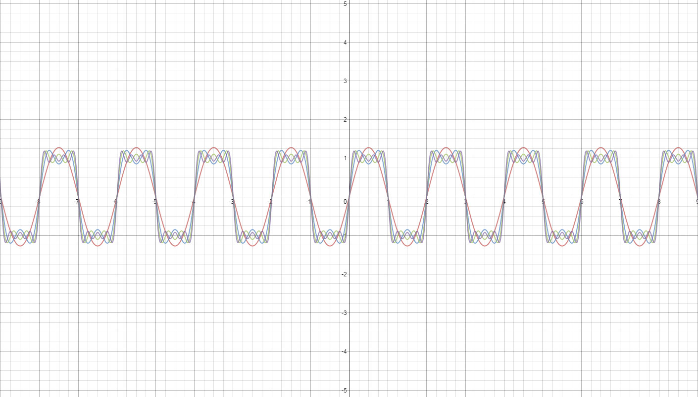
The importance of higher frequencies can be best illustrated with an example. In the case of an oscilloscope measuring and digitizing a square wave, very high frequencies are present. These are characteristic of rapidly changing levels, and a square wave is a great example. The Fourier series of a square wave is actually an infinite sum of sine waves, and this can be seen as the following series:

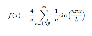
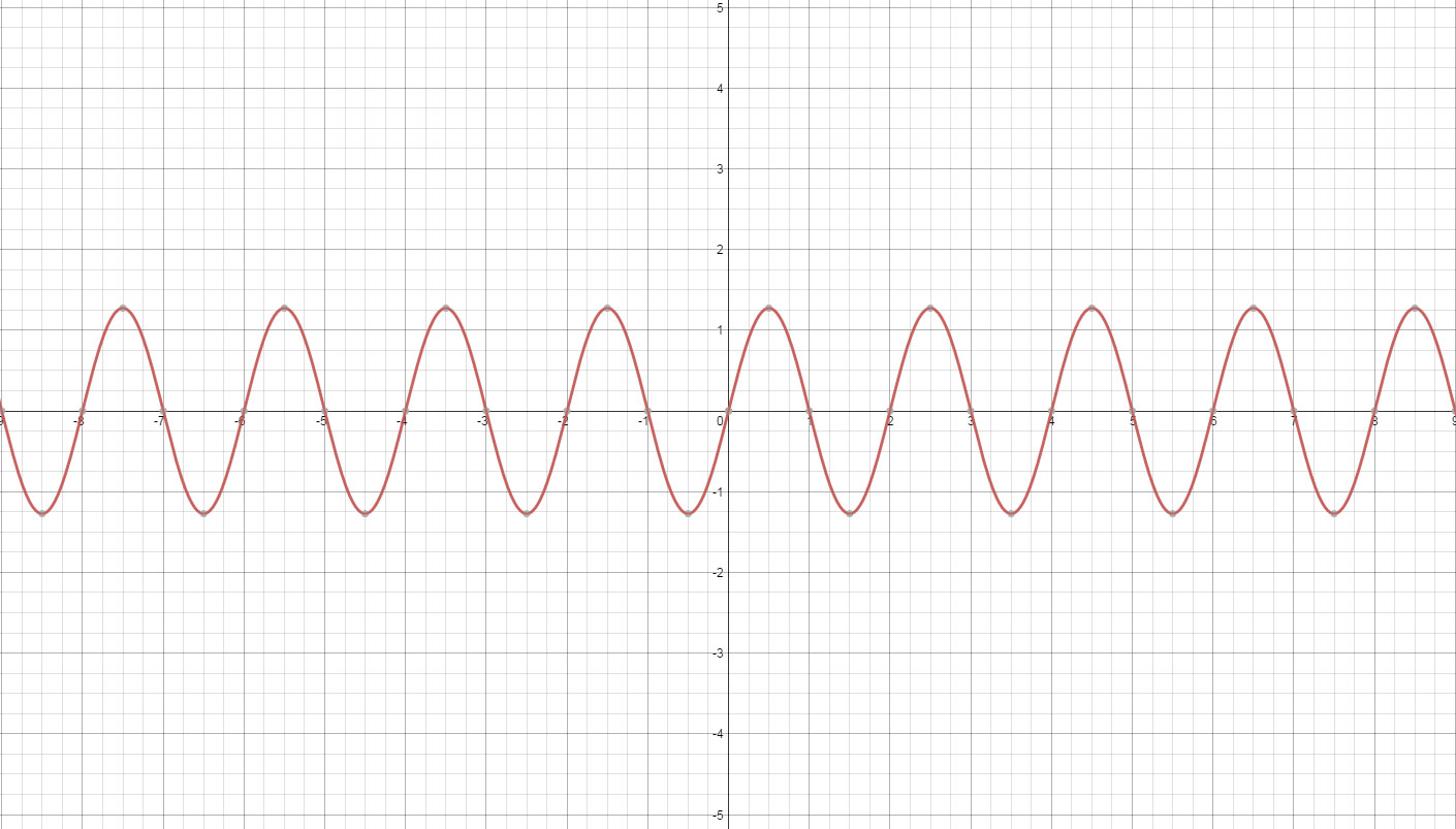
Figure 1 – Square wave Fourier series (1 component)

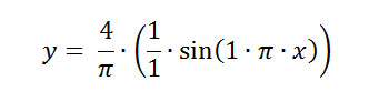
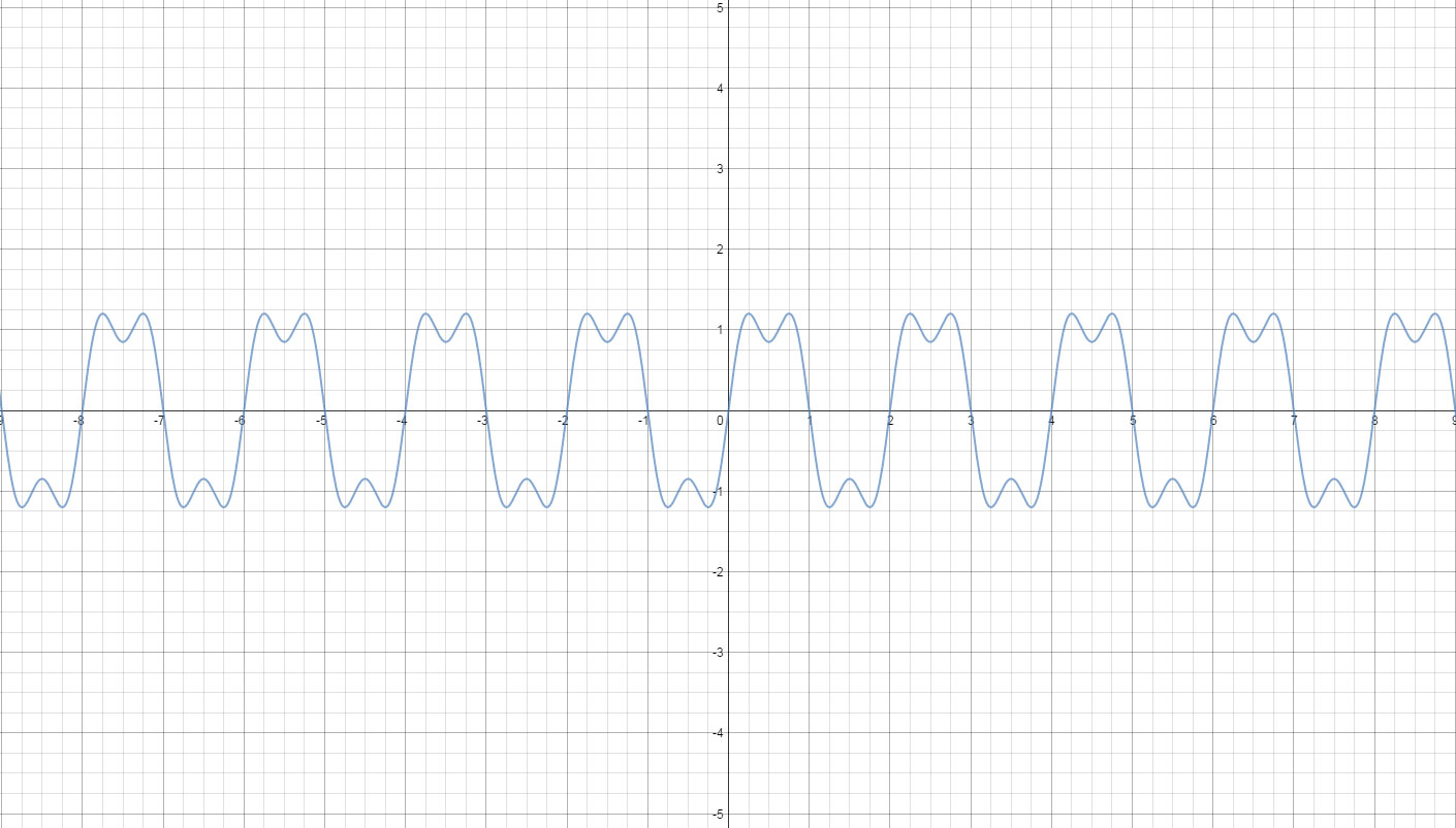
Figure 2 – Square wave Fourier series (2 components)

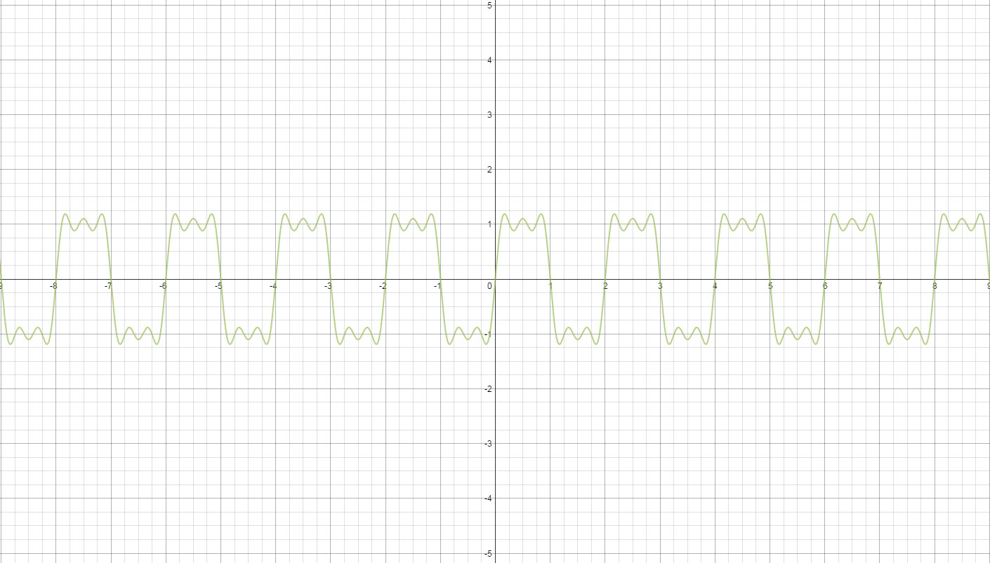
Figure 3 – Square wave Fourier series (3 components)

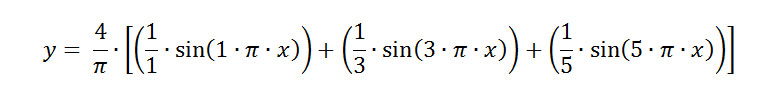
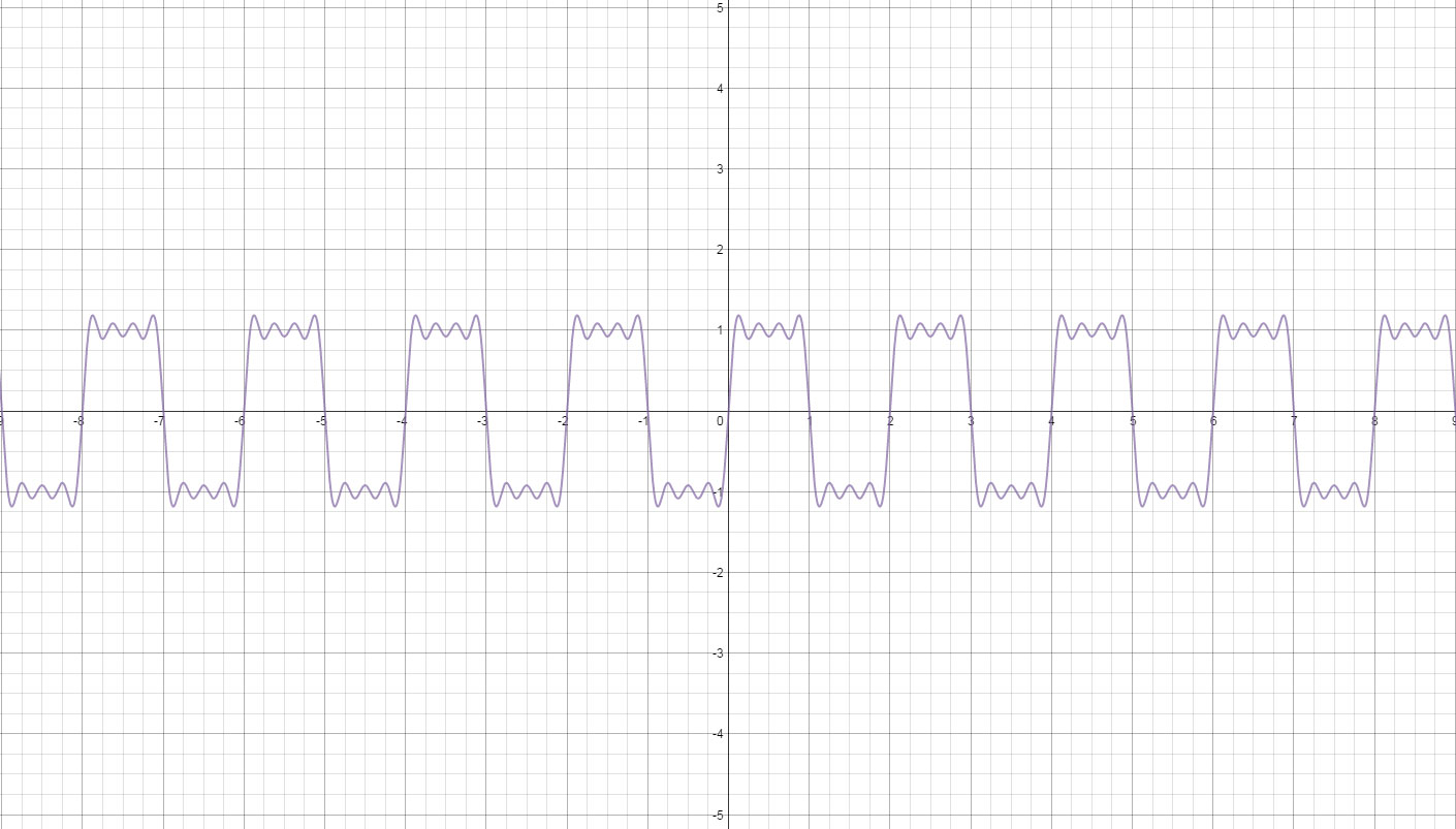
Figure 4 – Square wave Fourier series (4 components)

Figure 5 – Square wave Fourier series (5 components)

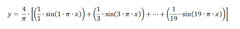
As can be seen, with each additional component, the signal becomes closer and closer to a perfect square wave. Naturally the frequency of each component is higher, and if we pass this through a low-pass filter, the higher frequencies will be omitted and we will be left with a much smoother wave without any sharp corners. This is one of the differences between a cheap oscilloscope and an expensive one with higher sampling rates and more memory – more accuracy will be achieved as higher frequencies will be picked up.
In the case of music, sharp sounds like the beating of a drum are likely to be composed of very high frequency components, and a digital conversion of low sampling rate is likely to produce very poor results. In these cases, an analogue recording will likely be a much better representation, which is why you may have heard people argue that the quality in a vinyl is superior to that of a digitally stored version.